Commonly Used Map Projections | Intergovernmental Committee on Surveying and Mapping

Introduction

Comparison of these projections:

Projection	Type	Key virtues	Comments
Stereographic	azimuthal	conformal	Created before 150 AD Best Used in areas over the Poles or for small scale continental mapping
Lambert Conformal Conic	conic	conformal	Created in 1772 Best Used in mid-latitudes – e.g. USA, Europe and Australia
Mercator	cylindrical	conformal and true direction	Created in 1569 Best Used in areas around the Equator and for marine navigation
Robinson	pseudo-cylindrical	all attributes are distorted to create a ‘more pleasant’ appearance	Created in the 1963 Best Used in areas around the Equator
Transverse Mercator	cylindrical	conformal	Created in 1772 Best Used for areas with a north-south orientation

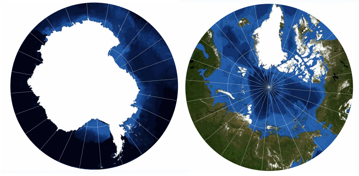
Azimuthal Projection – Stereographic

The oldest known record of this projection is from Ptolemy in about 150 AD. However it is believed that this projection was well known long before that time – probably as far back as the 2nd century BC.

Today, this is probably one of the most widely used Azimuthal projections. It is most commonly used over Polar areas, but can be used for small scale maps of continents such as Australia. The great attraction of the projection is that the Earth appears as if viewed form space or a globe.

This is a conformal projection in that shapes are well preserved over the map, although extreme distortions do occur towards the edge of the map. Directions are true from the centre of the map (the touch point of our imaginary ‘piece of paper’), but the map is not equal-area.

One interesting feature of the Stereographic projection is that any straight line which runs through the centre point is a Great Circle. The advantage of this is that for a place of interest (e.g. Canberra, the capital city of Australia) a map which uses the Stereographic projection and is centred on that place of interest true distances can be calculated to other places of interest (e.g. Canberra to Sydney; or Canberra to Darwin; or Canberra to Wellington, New Zealand).

These are two examples of maps using Stereographic projection over polar areas. In these the radiating lines are Great Circles. Projection information: Stereographic; centred on 140° East and 90° South (the South Pole) and 90° North (the North Pole), with a radius of 30° out from each Pole.

Stereographic Australia — Produced Using G.PROJECTOR – software developed by NASA and the Goddard Institute for Spatial Studies. Projection information: Stereographic; centred on 145° East and 30° South, with a radius of 30° out from the Pole. In this the Great Circles are not as obvious as with the two Polar maps above, but the same principle applies: any straight line which runs through the centre point is a Great Circle. This is an example of how a Great Circle does not have to be a set line of Longitude of Latitude.

Conic Projection – Lambert Conformal Conic

Johann Heinrich Lambert was a German ⁄ French mathematician and scientist. His mathematics was considered revolutionary for its time and is still considered important today. In 1772 he released both his Conformal Conic projection and the Transverse Mercator Projection.

Today the Lambert Conformal Conic projection has become a standard projection for mapping large areas (small scale) in the mid-latitudes – such as USA, Europe and Australia. It has also become particularly popular with aeronautical charts such as the 1:100,000 scale World Aeronautical Charts map series.

This projection commonly used two Standard Parallels (lines of latitudes which are unevenly spaced concentric circles).

The projection is conformal in that shapes are well preserved for a considerable extent near to the Standard Parallels. For world maps the shapes are extremely distorted away from Standard Parallels. This is why it is very popular for regional maps in mid-latitude areas (approximately 20° to 60° North and South).

Distances are only true along the Standard Parallels. Across the whole map directions are generally true.

Lambert projections — These two maps highlight the importance of selecting your Standard Parallel(s) carefully. For the first one the Standard Parallels are in the North and for the second they are in the South. Projection information: Lambert Conformal Conic; centred on 140° East and the Equator.
First map has standard Parallels at 30° and 60° South and the second has standard Parallels at 30° and 60° North.

Lambert Conformal Conic map of Australia — The Lambert Conformal Conic is the preferred projection for regional maps in mid-latitudes. In Australia the national mapping agency prefers to use this projection using 18° and 36° South as the two Standard Parallels. Projection information: Lambert Conformal Conic; centred on 140° East and 25° South, and two Standard Parallels 18° and 36° South.

Cylindrical Projection – Mercator

Notice the huge distortions in the Arctic and Antarctic regions, but the reasonable representation of landmasses out to about 50° north and south. Projection information: Mercator; centred on 140° East and the Standard Parallel is the Equator

One of the most famous map projections is the Mercator, created by a Flemish cartographer and geographer, Geradus Mercator in 1569.

It became the standard map projection for nautical purposes because of its ability to represent lines of constant true direction. (Constant true direction means that the straight line connecting any two points on the map is the same direction that a compass would show.) In an era of sailing ships and navigation based on direction only, this was a vitally important feature of this projection.

The Mercator Projection always has the Equator as its Standard Parallel. Its construction is such that the lines of longitude and latitude are at right angles to each other – this means that a world map is always a rectangle.

Also, the lines of longitude are evenly spaced apart. But the distance between the lines of latitude increase away from the Equator. This relationship is what allows the direction between any two points on the map to be constant true direction.

While this relationship between lines of lines of latitude and longitude correctly maintains direction, it allows for distortion to occur to areas, shapes and distances. Nearest the Equator there is little distortion. Distances along the Equator are always correct, but nowhere else on the map. Between about 15° north and south the areas and shapes are well preserved. Further out (to about 50° north and south) the areas and shapes are reasonably well preserved. This is why, for uses other than marine navigation, the Mercator projection is recommended for use in the Equatorial region only.

Despite these distortions the Mercator projection is generally regarded as being a conformal projection. This is because within small areas shapes are essentially true.

See also Transverse Mercator and Universal Transverse Mercator below.

Cylindrical Projection – Robinson

In the 1960s Arthur H. Robinson, a Wisconsin geography professor, developed a projection which has become much more popular than the Mercator projection for world maps. It was developed because modern map makers had become dissatisfied with the distortions inherent in the Mercator projection and they wanted a world projection which ‘looked’ more like reality.

In its time, the Robinson projection replaced the Mercator projection as the preferred projection for world maps. Major publishing houses which have used the Robinson projection include Rand McNally and National Geographic.

Robinson world map — Compare this to the Mercator projection map above. Projection information: Robinson; centred on 140° East and the Standard Parallel is the Equator.

As it is a pseudo-cylindrical projection, the Equator is its Standard Parallel and it still has similar distortion problems to the Mercator projection.

Between about 0° and 15° the areas and shapes are well preserved. However, the range of acceptable distortion has been expanded from approximately 15° north and south to approximately 45° north to south. Also, there is less distortion in the Polar regions.

Unlike the Mercator projection, the Robinson projection has both the lines of altitude and longitude evenly spaced across the map. The other significant difference to the Mercator is that only the line of longitude in the centre of the map is straight (Central Meridian), all others are curved, with the amount of curve increasing away from the Central Meridian.

In opting for a more pleasing appearance, the Robinson projection ‘traded’ off distortions – this projection is neither conformal, equal-area, equidistant nor true direction.

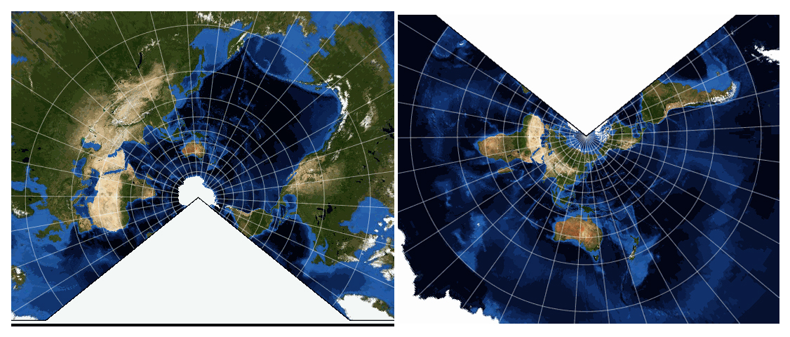
Cylindrical Projection – Transverse Mercator

The Transverse Mercator projection is based on the highly successful Mercator projection. The main strength of the Mercator projection is that it is highly accurate near the Equator (the ‘touch point’ of our imaginary piece of paper – otherwise called the Standard Parallel) and the main problem with the projection is that distortions increase away from the Equator. This set of virtues and vices meant that the Mercator projection is highly suitable for mapping places which have an east-west orientation near to the Equator but not suitable for mapping places which have are north-south orientation (eg South America or Chile).

Lambert’s stroke of genius was to change the way the imaginary piece of paper touched the Earth… instead of touching the Equator he had it touching a line of Longitude (any line of longitude). This touch point is called the Central Meridian of a map. This meant that accurate maps of places with north-south orientated places could now be produced. The map maker only needed to select a Central Meridian which ran through the middle of the map.

A Special Case – Universal Transverse Mercator System (UTM)

It took another 200 years for the next development in take place for the Mercator projection.

Again, like Lambert’s revolutionary change to the way that the Mercator projection was calculated; this development was a change in how the Transverse Mercator projection was used. In 1947 the North Atlantic Treaty Organisation (NATO) developed the Universal Transverse Mercator coordinate system (generally simply called UTM).

NATO recognised that the Mercator/Transverse Mercator projection was highly accurate along its Standard Parallel/Central Meridian. Indeed as far as 5° away from the Standard Parallel ⁄ Central Meridian there was minimal distortion.

Like the World Aeronautical Charts, the UTM system was able to build on the achievements of the International Map of the World. As well as developing an agreed, international specification the IMW had developed a regular grid system which covered the entire Surface of the Earth. For low to mid-latitudes (0° to 60° North and South) the IMW established a grid system that was 6° of longitude wide and 4° of latitude high.

Using this NATO designed a similar regular system for the Earth whereby it was divided into a series of 6° of longitudinal wide zones. There are a total of 60 longitudinal zones and these are numbered 1 to 60 – east from longitude 180° . These extend from the North Pole to the South Pole. A central meridian is placed in middle of each longitudinal zone. As a result, within a zone nothing is more than 3° from the central meridian and therefore locations, shapes and sizes and directions between all features are very accurate.

Please note that this is not a new ⁄ revised projection, but a series of maps using the same projection (Transverse Mercator). This is not commonly appreciated and UTM is often wrongly described as a projection in its own right – it is not – it is a projection system.

This is why UTM is regarded as a Special Case.

The shortcoming in the UTM system is that between these longitude zones directions are not true – this problem is overcome by ensuring that maps using the UTM system do not cover more than one zone.

World wide, including Australia, this UTM system is used by mapping agencies for local and national, topographic maps.

UTM Zones

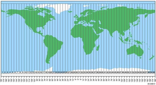
Compare this to the Mercator projection map above. Projection information: Robinson; centred on 140° East and the Standard Parallel is the Equator.

As already noted, the UTM system involves a series of longitudinal zones which are 6° wide and numbered 1 to 60 – east from longitude 180°.

However, unlike the International Map of the World (IMW) the UTM system opted to use latitudinal zones which were twice as wide – i.e. 8° of latitude wide. There are 20 of these and they are numbered A to Z (with O and I not being used) – north from Antarctica. Like the IMW system each feature on the Earth is now able to be described based on the UTM grid it is located in. One confusing item is that these grid cells are variably called a UTM zone.

For example, in the case of Sydney, Australia, its UTM grid cell (zone) would be identified as:

H – for the latitudinal zone it belongs to
56 – for the longitudinal zone it belongs to

Add the two together – the UTM grid zone (grid cell) which contains Sydney is 56H

UTM Map grid and the Australian Map Grid

As is explained in the section tiled Explaining Some Jargon – Graticules and Grids there is a significant difference between the two.

Graticules are lines of Longitude and Latitude. These never form a square or rectangular shape and their shape changes dramatically from the Equator to the Pole – from being close to square shaped to being close to triangle shaped.
Grids are a regularly shaped overlay to a map. They are usually square, but they may be rectangular.

Grids rarely run parallel to lines of Longitude and Latitude.

Besides ease of use, there is another advantage to a grid – on any given map it always covers the same amount of the Earth’s surface. This is not true of a graticule system! A 1° x1° block of latitude and longitude near the Equator will always cover vastly more of the Earth’s surface and a 1° x1° block closer to a Pole. Therefore it is easy to measure distances using a grid – it removes the foibles of distortions inherent in each map projection.

When NATO created the UTM system it recognised this fact and built a grid system into it. This involves a regular and complex system of letters to identify grid cells. To identify individual features or locations distances are first measured from the west to the feature and then measured from the south to the feature. The three are combined to give a precise location – based on the map grid.

Explaining some jargon:

The Australian Map Grid (AMG) is the map grid which had been developed as part of the UTM system to best suit Australian needs.
Northings – these are the horizontal parallel lines of the grid – i.e. they are series of lines which run from the west to the east (similar to lines of latitude – but not the same). Their values increase towards the north.
Eastings – these are the vertical parallel lines of the grid – i.e. they are series of lines which run from the north to south (similar to lines of longitude – but not the same). Their values increase towards the east.

A Special Case – Geographic (or Plate Carrée)

This is a mathematically simple projection. It is also an ancient projection (possibly developed by Marinus of Tyre in 100).

Because of its simplicity it was commonly used in the past (before computers allowed for very complex calculations) and it has been adopted as the projection of choice for use in computer mapping applications – notably Geographic Information Systems (GIS) and on web pages. Also, again because of its simplicity, it is equally able to be used with world and regional maps.

Plate Carrée is the French term for flat square. In GIS operations this projection is commonly referred to as Geographicals.

This is a cylindrical projection, with the Equator as its Standard Parallel. The difference with this projection is that the latitude and longitude lines intersect to form regularly sized squares. By way of comparison, in the Mercator and Robinson projections they form irregularly sized rectangles.

While we have described the Geographic or Plate Carrée as a projection, there is some debate as to whether it should be considered to be a projection. This is because it makes no attempt to compensate for distortions due to the transfer of information from the surface of the Earth onto a ‘flat piece of paper’ (our map).

This is why we are describing the Geographical projection as a Special Case.

Refer to the section on Projections for more information about distortions generated by projections.